LLMS and other foundation models are capable of accomplishing a wide range of tasks. However, we may have a task that they do not perform well off the shelf. In principle, we can address this problem by fine tuning a model for that task. However, fine tuning foundation models is extremely expensive.

Parameter-efficient fine tuning (PEFT) is meant to address this problem. Rather than adjusting all of the weights of a model, it adds relatively small adapters to the model and trains those adapters on new data.

This post implements a few parameter efficient fine tuning techniques: LORA, DORA, and RS-LORA. It illustrates these methods on a simple regression problem in which we adapt a model that has been trained on a quadratic data set to a cubic data set. These polynomial fitting problems are many orders of magnitude simpler than language modeling, so the way these PEFT methods behave on them may not tell us much about how they behave when applied to foundation models. However, the illustrations do illustrate the general concepts of full and parameter-efficient fine tuning and help confirm that the methods are working as expected.

The LoRA and DoRA are implementations adapted from Sebastian Raschka’s Improving LoRA: Implementing Weight-Decomposed Low-Rank Adaptation (DoRA) from Scratch. The visualization methods are adapted from Jeremy Howard’s FastAI v3 Lesson 2: SGD. Both were published under the Apache License 2.0.

Setup

import copy
from functools import partial
from pathlib import Path
from typing import Optional

from IPython.display import HTML
from matplotlib import animation
import matplotlib.pyplot as plt
import numpy as np
import torch
from torch import Tensor
import torch.nn as nn
import torch.nn.functional as F

mps_available = torch.backends.mps.is_available()
mps_available

True

def set_seeds(seed=42):
    torch.manual_seed(seed)
    np.random.seed(seed)

    if torch.cuda.is_available():
        torch.cuda.manual_seed_all(seed)
    if torch.backends.mps.is_available():
        torch.mps.manual_seed(seed)

    torch.backends.cudnn.deterministic = True
    torch.backends.cudnn.benchmark = False


set_seeds()

# Model Configuration
RANK = 4  # LoRA/DoRA rank
ALPHA = 32  # LoRA/DoRA scaling factor
NUM_HIDDEN_1 = 20
NUM_HIDDEN_2 = 20

# Training Configuration
LEARNING_RATE = 0.01
NUM_STEPS = 150

# Animation Configuration
INTERVAL = 20
OUTPUT_DIR = Path("output")
OUTPUT_DIR.mkdir(parents=True, exist_ok=True)

# Data Configuration
NUM_SAMPLES = 100
NOISE_SCALE = 0.1

torch.__version__

'2.6.0'

def get_device() -> torch.device:
    """Determine the best available device for PyTorch."""
    if torch.cuda.is_available():
        print("Using CUDA device")
        return torch.device("cuda")
    elif torch.backends.mps.is_available():
        print("Using MPS device")
        return torch.device("mps")
    else:
        print("Using CPU device")
        return torch.device("cpu")


DEVICE = get_device()
DEVICE

Using MPS device

device(type='mps')

Generate Data

def generate_data(
    num_samples: int = NUM_SAMPLES,
    noise_scale: float = NOISE_SCALE,
    device: Optional[torch.device] = None,
) -> tuple[Tensor, Tensor, Tensor]:
    """Generate synthetic data for training.

    Args:
        num_samples: Number of data points to generate
        noise_scale: Scale of random noise to add
        device: Device to place tensors on

    Returns:
        x: Input tensor
        y1: First target tensor
        y2: Second target tensor
    """
    if device is None:
        device = get_device()

    try:
        x = torch.linspace(-1, 1, num_samples)[:, None].to(device)
        noise = torch.randn(num_samples)[:, None].to(device)

        y1 = x**2 + noise_scale * noise
        y2 = (
            x**3
            - 0.5 * x**2
            + 0.5
            + noise_scale * torch.randn(num_samples)[:, None].to(device)
        )

        return x, y1, y2
    except RuntimeError as e:
        print(f"Error generating data: {e}")
        raise


x, y1, y2 = generate_data(device=DEVICE)

Train Base Model

Training a multilayer perceptron on the quadratic data set.

class MultilayerPerceptron(nn.Module):
    def __init__(self, num_features, num_hidden_1, num_hidden_2, device=None):
        super().__init__()
        if device is None:
            device = get_device()

        self.layers = nn.Sequential(
            nn.Linear(num_features, num_hidden_1),
            nn.ReLU(),
            nn.Linear(num_hidden_1, num_hidden_2),
            nn.ReLU(),
            nn.Linear(num_hidden_2, 1),
        ).to(device)

    def forward(self, x):
        return self.layers(x)

model = MultilayerPerceptron(1, NUM_HIDDEN_1, NUM_HIDDEN_2).to(DEVICE)
model

Using MPS device

MultilayerPerceptron(
  (layers): Sequential(
    (0): Linear(in_features=1, out_features=20, bias=True)
    (1): ReLU()
    (2): Linear(in_features=20, out_features=20, bias=True)
    (3): ReLU()
    (4): Linear(in_features=20, out_features=1, bias=True)
  )
)

def create_training_plot(x, y1, y2, model_output):
    """Create a scatter plot of the data points and model prediction line.

    Args:
        x: Input tensor
        y1: First dataset tensor
        y2: Second dataset tensor
        model_output: Model predictions tensor

    Returns:
        fig: matplotlib figure
        line: Line artist for model predictions
    """
    x_cpu = x.cpu()
    y1_cpu = y1.cpu()
    y2_cpu = y2.cpu()
    output_cpu = model_output.cpu().detach()

    fig = plt.figure()
    plt.scatter(x_cpu, y1_cpu, label="Dataset 1")
    plt.scatter(x_cpu, y2_cpu, label="Dataset 2")
    (line,) = plt.plot(x_cpu, output_cpu, "r-", label="Model Prediction")
    plt.legend()
    return fig, line


def animate(model, y, optimizer, line, frame):
    """Animate one frame of training.

    Args:
        model: PyTorch model to train
        y: Target tensor
        optimizer: PyTorch optimizer
        line: Line artist to update
        frame: Current frame number
    """
    # FuncAnimation calls frame=0 twice at start, we want to show initial state both times
    if frame == 0:
        line.set_ydata(model(x).cpu().detach().numpy())
        print(f"Initial Loss: {nn.MSELoss()(model(x), y):.4f}")
        return (line,)

    loss = update(model, y, optimizer)
    if frame % 10 == 0:
        print(f"Iteration {frame}, Loss: {loss:.4f}")

    line.set_ydata(model(x).cpu().detach().numpy())
    return (line,)


def update(model, y, optimizer, loss_fn=nn.MSELoss()):
    """Perform one training step."""
    optimizer.zero_grad()
    try:
        y_pred = model(x)
        loss = loss_fn(y_pred, y)
        loss.backward()
        optimizer.step()
        return loss.item()
    except RuntimeError as e:
        print(f"Error during training step: {e}")
        raise


def create_training_animation(
    model, x, y, optimizer, NUM_STEPS=NUM_STEPS, interval=INTERVAL
):
    """Create an animation of the training process.

    Args:
        model: PyTorch model to train
        x: Input tensor
        y: Target tensor
        optimizer: PyTorch optimizer
        NUM_STEPS: Number of training steps to animate
        interval: Milliseconds between animation frames
    """
    fig, line = create_training_plot(x, y1, y2, model(x))
    plt.close()  # Prevent display of initial figure

    anim = animation.FuncAnimation(
        fig,
        partial(animate, model, y, optimizer, line),
        frames=NUM_STEPS,
        repeat=False,
        interval=interval,
    )

    return anim

anim = create_training_animation(
    model,
    x,
    y1,
    torch.optim.Adam(model.parameters(), lr=LEARNING_RATE),
)
HTML(anim.to_html5_video())

Initial Loss: 0.1330
Initial Loss: 0.1330
Iteration 10, Loss: 0.0679
Iteration 20, Loss: 0.0158
Iteration 30, Loss: 0.0142
Iteration 40, Loss: 0.0109
Iteration 50, Loss: 0.0093
Iteration 60, Loss: 0.0089
Iteration 70, Loss: 0.0087
Iteration 80, Loss: 0.0086
Iteration 90, Loss: 0.0085
Iteration 100, Loss: 0.0084
Iteration 110, Loss: 0.0084
Iteration 120, Loss: 0.0083
Iteration 130, Loss: 0.0082
Iteration 140, Loss: 0.0082

Full Fine Tuning

Fine tune that model on the cubic data set in the standard way. This approach works fine on this simple problem but is often prohibitively expensive for foundation models.

finetune_model = copy.deepcopy(model)

anim = create_training_animation(
    finetune_model,
    x,
    y2,
    torch.optim.Adam(finetune_model.parameters(), lr=LEARNING_RATE),
)
HTML(anim.to_html5_video())

Initial Loss: 0.3533
Initial Loss: 0.3533
Iteration 10, Loss: 0.0699
Iteration 20, Loss: 0.0476
Iteration 30, Loss: 0.0357
Iteration 40, Loss: 0.0283
Iteration 50, Loss: 0.0235
Iteration 60, Loss: 0.0193
Iteration 70, Loss: 0.0154
Iteration 80, Loss: 0.0122
Iteration 90, Loss: 0.0102
Iteration 100, Loss: 0.0090
Iteration 110, Loss: 0.0085
Iteration 120, Loss: 0.0082
Iteration 130, Loss: 0.0079
Iteration 140, Loss: 0.0077

LoRA Fine Tuning

Instead of tuning all the weights of a given linear layer, LoRA adds an adapter to that layer with a smaller number of parameters and then tunes just those parameters.

Our model expands the input x to 20 dimensions, passes those 20 dimensions through a linear layer, and then reduces the result back down to a single output y, with intermediate ReLU nonlinearities:

model

MultilayerPerceptron(
  (layers): Sequential(
    (0): Linear(in_features=1, out_features=20, bias=True)
    (1): ReLU()
    (2): Linear(in_features=20, out_features=20, bias=True)
    (3): ReLU()
    (4): Linear(in_features=20, out_features=1, bias=True)
  )
)

The middle layer \(W\) (shown above as (2): Linear(in_features=20, out_features=20, bias=True)) has 400 parameters (ignoring the bias):

plt.imshow(model.layers[2].weight.detach().cpu().numpy())
plt.title("Weight matrix for middle layer")
plt.xticks([])
plt.yticks([])
plt.show()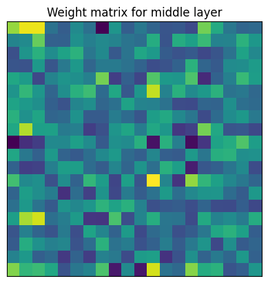

Full fine tuning adjusts all 400 of these parameters.

class LoRALayer(nn.Module):
    def __init__(self, in_dim: int, out_dim: int, rank: int, alpha: float) -> None:
        super().__init__()
        std_dev = 1 / torch.sqrt(torch.tensor(rank).float())
        self.A = nn.Parameter(torch.randn(in_dim, rank) * std_dev)
        self.B = nn.Parameter(torch.zeros(rank, out_dim))
        self.gamma_r = alpha / rank

    def forward(self, x: Tensor) -> Tensor:
        # https://magazine.sebastianraschka.com/p/lora-and-dora-from-scratch
        # uses alpha directly here in place of gamma_r, but using gamma_r
        # makes it simpler to compare LoRA and rsLoRA.
        return self.gamma_r * (x @ self.A @ self.B)

LoRA with rank 4 instead creates a tall and skinny matrix \(A\) with 20 rows and 4 columns and a wide and short matrix \(B\) with 4 rows and 20 columns. (The rank is a hyperparameter that we choose; higher rank makes the adapter more expressive but increases the number of parameters to tune, bringing us closer to full fine tuning.) The product of those matrices is still 20x20, so we can add it to our original matrix, but it has 2x4x20 = 160 parameters to tune instead of 400.

\(B\) is initialized to zero, so the initial output of the model is the same as it would be without the LoRA layer.

fig, ax = plt.subplots(1, 3, figsize=(15, 5))
lora_layer = LoRALayer(20, 20, 4, 32)
ax[0].imshow(lora_layer.A.detach().cpu().numpy())
ax[0].set_title("LoRA A matrix")
ax[0].set_xticks([])
ax[0].set_yticks([])
ax[1].imshow(lora_layer.B.detach().cpu().numpy())
ax[1].set_title("@ LoRA B matrix")
ax[1].set_xticks([])
ax[1].set_yticks([])
ax[2].imshow(lora_layer.A.detach().cpu().numpy() @ lora_layer.B.detach().cpu().numpy())
ax[2].set_title("= LoRA matrix")
ax[2].set_xticks([])
ax[2].set_yticks([])
ax[2].set_aspect("equal")
plt.show()

class LinearWithLoRA(nn.Module):
    def __init__(
        self,
        linear: nn.Linear,
        rank: int,
        alpha: float,
        lora_layer_class: nn.Module = LoRALayer,
    ) -> None:
        super().__init__()
        self.linear = linear
        self.lora = lora_layer_class(
            linear.in_features, linear.out_features, rank, alpha
        )

    def forward(self, x: Tensor) -> Tensor:
        return self.linear(x) + self.lora(x)

def test_lora_layer_does_not_change_initial_output():
    layer = nn.Linear(1, 2).to(DEVICE)
    original_output = layer(x[0])
    layer_lora = LinearWithLoRA(layer, rank=1, alpha=4).to(DEVICE)
    lora_output = layer_lora(x[0])
    assert (lora_output == original_output).all()


test_lora_layer_does_not_change_initial_output()

The implementation above passes the inputs through the original linear layer and the LoRA layer separately (i.e. does matrix multiplication with each) and then adds the results.

We could save computation by adding the original linear layer and the LoRA layer first and then doing one matrix multiplication, as follows:

class LinearWithLoRAMerged(LinearWithLoRA):
    def forward(self, x):
        lora = self.lora.A @ self.lora.B
        combined_weight = self.linear.weight + self.lora.gamma_r * lora.T
        return F.linear(x, combined_weight, self.linear.bias)

def test_lora_merged_layer_does_not_change_initial_output():
    layer = nn.Linear(1, 2).to(DEVICE)
    original_output = layer(x[0])
    layer_lora = LinearWithLoRAMerged(layer, rank=1, alpha=4).to(DEVICE)
    lora_output = layer_lora(x[0])
    assert (lora_output == original_output).all()


test_lora_merged_layer_does_not_change_initial_output()

After training, we could merge the original and LoRA layers permanently into a new linear layer. That approach would save still more computation at prediction time. However, it would prevent us from recovering the original model by removing the LoRA layers. We will not implement that approach here.

Let’s fine tune these two LoRA implementations on the cubic data set and confirm that they give the same results.

def freeze_linear_layers(model):
    for child in model.children():
        if isinstance(child, nn.Linear):
            for param in child.parameters():
                param.requires_grad = False
        else:
            freeze_linear_layers(child)

def create_lora_model(
    base_model,
    lora_layer_indices,
    lora_layer_class,
):
    """Create a LoRA version of a base model.

    Args:
        base_model: Base model to apply LoRA to
        lora_layer_indices: Indices of the layers to apply LoRA to
        lora_layer_class: Class of the LoRA layer to use

    Returns:
        Modified model with LoRA layers
    """
    lora_model = copy.deepcopy(base_model)

    for index in lora_layer_indices:
        lora_model.layers[index] = lora_layer_class(lora_model.layers[index]).to(DEVICE)

    freeze_linear_layers(lora_model)

    return lora_model

torch.manual_seed(
    678
)  # resetting seed so LoRA and LoRAMerged get the same LoRA weight initializations
lora_model = create_lora_model(
    model,
    lora_layer_indices=[2],
    lora_layer_class=partial(LinearWithLoRA, rank=RANK, alpha=ALPHA),
)

lora_model

MultilayerPerceptron(
  (layers): Sequential(
    (0): Linear(in_features=1, out_features=20, bias=True)
    (1): ReLU()
    (2): LinearWithLoRA(
      (linear): Linear(in_features=20, out_features=20, bias=True)
      (lora): LoRALayer()
    )
    (3): ReLU()
    (4): Linear(in_features=20, out_features=1, bias=True)
  )
)

print("Confirming LoRA model linear layers are frozen")
for name, param in lora_model.named_parameters():
    print(f"{name}: {param.requires_grad}")

Confirming LoRA model linear layers are frozen
layers.0.weight: False
layers.0.bias: False
layers.2.linear.weight: False
layers.2.linear.bias: False
layers.2.lora.A: True
layers.2.lora.B: True
layers.4.weight: False
layers.4.bias: False

torch.manual_seed(
    678
)  # resetting seed so LoRA and LoRAMerged get the same LoRA weight initializations
lora_model_merged = create_lora_model(
    model,
    lora_layer_indices=[2],
    lora_layer_class=partial(LinearWithLoRAMerged, rank=RANK, alpha=ALPHA),
)

lora_model_merged

MultilayerPerceptron(
  (layers): Sequential(
    (0): Linear(in_features=1, out_features=20, bias=True)
    (1): ReLU()
    (2): LinearWithLoRAMerged(
      (linear): Linear(in_features=20, out_features=20, bias=True)
      (lora): LoRALayer()
    )
    (3): ReLU()
    (4): Linear(in_features=20, out_features=1, bias=True)
  )
)

print("Confirming LoRA Merged model linear layers are frozen")
for name, param in lora_model_merged.named_parameters():
    print(f"{name}: {param.requires_grad}")

Confirming LoRA Merged model linear layers are frozen
layers.0.weight: False
layers.0.bias: False
layers.2.linear.weight: False
layers.2.linear.bias: False
layers.2.lora.A: True
layers.2.lora.B: True
layers.4.weight: False
layers.4.bias: False

def test_lora_models_produce_same_output():
    with torch.no_grad():
        output1 = lora_model(x)
        output2 = lora_model_merged(x)
        diff = (output1 - output2).abs().max().item()
        assert diff < 1e-5


test_lora_models_produce_same_output()

anim = create_training_animation(
    lora_model,
    x,
    y2,
    torch.optim.Adam(lora_model.parameters(), lr=LEARNING_RATE),
)
HTML(anim.to_html5_video())

Initial Loss: 0.3533
Initial Loss: 0.3533
Iteration 10, Loss: 0.0761
Iteration 20, Loss: 0.0494
Iteration 30, Loss: 0.0287
Iteration 40, Loss: 0.0241
Iteration 50, Loss: 0.0183
Iteration 60, Loss: 0.0154
Iteration 70, Loss: 0.0138
Iteration 80, Loss: 0.0130
Iteration 90, Loss: 0.0126
Iteration 100, Loss: 0.0124
Iteration 110, Loss: 0.0122
Iteration 120, Loss: 0.0121
Iteration 130, Loss: 0.0119
Iteration 140, Loss: 0.0118

anim = create_training_animation(
    lora_model_merged,
    x,
    y2,
    torch.optim.Adam(lora_model_merged.parameters(), lr=LEARNING_RATE),
)
HTML(anim.to_html5_video())

Initial Loss: 0.3533
Initial Loss: 0.3533
Iteration 10, Loss: 0.0761
Iteration 20, Loss: 0.0494
Iteration 30, Loss: 0.0287
Iteration 40, Loss: 0.0241
Iteration 50, Loss: 0.0183
Iteration 60, Loss: 0.0154
Iteration 70, Loss: 0.0138
Iteration 80, Loss: 0.0130
Iteration 90, Loss: 0.0126
Iteration 100, Loss: 0.0124
Iteration 110, Loss: 0.0122
Iteration 120, Loss: 0.0121
Iteration 130, Loss: 0.0119
Iteration 140, Loss: 0.0118

Here are the LoRA matrices after training:

fig, ax = plt.subplots(1, 3, figsize=(15, 5))
ax[0].imshow(lora_model.layers[2].lora.A.detach().cpu().numpy())
ax[0].set_title("LoRA A matrix")
ax[0].set_xticks([])
ax[0].set_yticks([])
ax[1].imshow(lora_model.layers[2].lora.B.detach().cpu().numpy())
ax[1].set_title("@ LoRA B matrix")
ax[1].set_xticks([])
ax[1].set_yticks([])
ax[2].imshow(
    lora_model.layers[2].lora.A.detach().cpu().numpy()
    @ lora_model.layers[2].lora.B.detach().cpu().numpy()
)
ax[2].set_title("= LoRA matrix")
ax[2].set_xticks([])
ax[2].set_yticks([])
ax[2].set_aspect("equal")
plt.savefig("posts/2025-02-14_fine-tuning-on-regression-task/lora_matrices.png")
plt.show()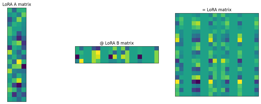

DoRA Fine-Tuning

DoRA is similar to LoRA. However, it combines the linear and LoRA weights and then applies weight normalization; that is, it reparameterizes the combined weight matrix into a directional component and a scaling factor. The result is mathematically equivalent to a LoRA model in the forward pass, but it has been observed to train better.

class LinearWithDoRAMerged(nn.Module):
    def __init__(self, linear, rank, alpha):
        super().__init__()
        self.linear = linear
        self.lora = LoRALayer(linear.in_features, linear.out_features, rank, alpha)
        self.m = nn.Parameter(self.linear.weight.norm(p=2, dim=0, keepdim=True))

    def forward(self, x):
        lora = self.lora.A @ self.lora.B
        numerator = self.linear.weight + self.lora.gamma_r * lora.T
        denominator = numerator.norm(p=2, dim=0, keepdim=True)
        directional_component = numerator / denominator
        new_weight = self.m * directional_component
        return F.linear(x, new_weight, self.linear.bias)

dora_model = create_lora_model(
    model,
    lora_layer_indices=[2],
    lora_layer_class=partial(LinearWithDoRAMerged, rank=RANK, alpha=ALPHA),
)

dora_model

MultilayerPerceptron(
  (layers): Sequential(
    (0): Linear(in_features=1, out_features=20, bias=True)
    (1): ReLU()
    (2): LinearWithDoRAMerged(
      (linear): Linear(in_features=20, out_features=20, bias=True)
      (lora): LoRALayer()
    )
    (3): ReLU()
    (4): Linear(in_features=20, out_features=1, bias=True)
  )
)

for name, param in dora_model.named_parameters():
    print(f"{name}: {param.requires_grad}")

layers.0.weight: False
layers.0.bias: False
layers.2.m: True
layers.2.linear.weight: False
layers.2.linear.bias: False
layers.2.lora.A: True
layers.2.lora.B: True
layers.4.weight: False
layers.4.bias: False

anim = create_training_animation(
    dora_model,
    x,
    y2,
    torch.optim.Adam(dora_model.parameters(), lr=LEARNING_RATE),
)
HTML(anim.to_html5_video())

Initial Loss: 0.3533
Initial Loss: 0.3533
Iteration 10, Loss: 0.0456
Iteration 20, Loss: 0.0318
Iteration 30, Loss: 0.0243
Iteration 40, Loss: 0.0197
Iteration 50, Loss: 0.0168
Iteration 60, Loss: 0.0148
Iteration 70, Loss: 0.0135
Iteration 80, Loss: 0.0128
Iteration 90, Loss: 0.0123
Iteration 100, Loss: 0.0120
Iteration 110, Loss: 0.0117
Iteration 120, Loss: 0.0114
Iteration 130, Loss: 0.0112
Iteration 140, Loss: 0.0110

rsLoRA Fine-Tuning

When it combines the linear and adapter weights, LoRA scales the adapter weights by \(\frac{\alpha}{r}\), where \(\alpha\) is a hyperparameter scaling factor and \(r\) is the rank of the LoRA layer. Reducing the scaling factor as we increase the rank ensures that the adapter weights do not grow too large as the rank increases.

A Rank Stabilization Scaling Factor for Fine-Tuning with LoRA showed keeping training stable for large ranks requires scaling the adapter weights by \(\frac{\alpha}{\sqrt{r}}\) rather than \(\frac{\alpha}{r}\). rsLoRA is just LoRA with this modified scaling factor.

class RsLoRALayer(LoRALayer):
    def __init__(self, in_dim: int, out_dim: int, rank: int, alpha: float) -> None:
        super().__init__(in_dim, out_dim, rank, alpha)
        self.gamma_r = alpha / (rank**1 / 2)

Reproduce LoRA results

Let’s implement rsLoRA, but initially adjust \(\alpha\) to get the same scaling factor as before, so that we should get the same results as with LoRA.

torch.manual_seed(
    678
)  # resetting seed so we get the same LoRA weight initializations as before
rslora_model = create_lora_model(
    model,
    lora_layer_indices=[2],
    lora_layer_class=partial(
        LinearWithLoRA,
        rank=RANK,
        # will give same gamma_r as LoRA above, so should train the same
        alpha=ALPHA / (RANK**1 / 2),
        lora_layer_class=RsLoRALayer,
    ),
)
rslora_model

MultilayerPerceptron(
  (layers): Sequential(
    (0): Linear(in_features=1, out_features=20, bias=True)
    (1): ReLU()
    (2): LinearWithLoRA(
      (linear): Linear(in_features=20, out_features=20, bias=True)
      (lora): RsLoRALayer()
    )
    (3): ReLU()
    (4): Linear(in_features=20, out_features=1, bias=True)
  )
)

for name, param in rslora_model.named_parameters():
    print(f"{name}: {param.requires_grad}")

layers.0.weight: False
layers.0.bias: False
layers.2.linear.weight: False
layers.2.linear.bias: False
layers.2.lora.A: True
layers.2.lora.B: True
layers.4.weight: False
layers.4.bias: False

anim = create_training_animation(
    rslora_model,
    x,
    y2,
    torch.optim.Adam(rslora_model.parameters(), lr=LEARNING_RATE),
)
HTML(anim.to_html5_video())

Initial Loss: 0.3533
Initial Loss: 0.3533
Iteration 10, Loss: 0.0761
Iteration 20, Loss: 0.0494
Iteration 30, Loss: 0.0287
Iteration 40, Loss: 0.0241
Iteration 50, Loss: 0.0183
Iteration 60, Loss: 0.0154
Iteration 70, Loss: 0.0138
Iteration 80, Loss: 0.0130
Iteration 90, Loss: 0.0126
Iteration 100, Loss: 0.0124
Iteration 110, Loss: 0.0122
Iteration 120, Loss: 0.0121
Iteration 130, Loss: 0.0119
Iteration 140, Loss: 0.0118

Compare LoRA and rsLoRA at Extreme Ranks

Now let’s keep \(\alpha\) the same and see how LoRA and rsLoRA perform at extreme ranks. I would not necessarily expect rsLoRA to perform better than LoRA at extreme ranks in this simple case, but at least we can illustrate the type of situation in which rsLoRA is expected to perform better.

LoRA at Low Rank

lora_model = create_lora_model(
    model,
    lora_layer_indices=[2],
    lora_layer_class=partial(LinearWithLoRAMerged, rank=1, alpha=ALPHA),
)
anim = create_training_animation(
    lora_model,
    x,
    y2,
    torch.optim.Adam(lora_model.parameters(), lr=LEARNING_RATE),
)
HTML(anim.to_html5_video())

Initial Loss: 0.3533
Initial Loss: 0.3533
Iteration 10, Loss: 0.0739
Iteration 20, Loss: 0.0678
Iteration 30, Loss: 0.0291
Iteration 40, Loss: 0.0260
Iteration 50, Loss: 0.0236
Iteration 60, Loss: 0.0209
Iteration 70, Loss: 0.0195
Iteration 80, Loss: 0.0186
Iteration 90, Loss: 0.0177
Iteration 100, Loss: 0.0170
Iteration 110, Loss: 0.0167
Iteration 120, Loss: 0.0164
Iteration 130, Loss: 0.0163
Iteration 140, Loss: 0.0162

LoRA at High Rank

lora_model = create_lora_model(
    model,
    lora_layer_indices=[2],
    lora_layer_class=partial(LinearWithLoRAMerged, rank=20, alpha=ALPHA),
)
anim = create_training_animation(
    lora_model,
    x,
    y2,
    torch.optim.Adam(lora_model.parameters(), lr=LEARNING_RATE),
)
HTML(anim.to_html5_video())

Initial Loss: 0.3533
Initial Loss: 0.3533
Iteration 10, Loss: 0.0561
Iteration 20, Loss: 0.0304
Iteration 30, Loss: 0.0235
Iteration 40, Loss: 0.0161
Iteration 50, Loss: 0.0137
Iteration 60, Loss: 0.0130
Iteration 70, Loss: 0.0125
Iteration 80, Loss: 0.0121
Iteration 90, Loss: 0.0118
Iteration 100, Loss: 0.0116
Iteration 110, Loss: 0.0115
Iteration 120, Loss: 0.0113
Iteration 130, Loss: 0.0113
Iteration 140, Loss: 0.0112

rsLoRA at Low Rank

rslora_model = create_lora_model(
    model,
    lora_layer_indices=[2],
    lora_layer_class=partial(
        LinearWithLoRA,
        rank=1,
        alpha=ALPHA,
        lora_layer_class=RsLoRALayer,
    ),
)
anim = create_training_animation(
    rslora_model,
    x,
    y2,
    torch.optim.Adam(rslora_model.parameters(), lr=LEARNING_RATE),
)
HTML(anim.to_html5_video())

Initial Loss: 0.3533
Initial Loss: 0.3533
Iteration 10, Loss: 0.1752
Iteration 20, Loss: 0.1717
Iteration 30, Loss: 0.1737
Iteration 40, Loss: 0.1724
Iteration 50, Loss: 0.1708
Iteration 60, Loss: 0.1691
Iteration 70, Loss: 0.1666
Iteration 80, Loss: 0.1623
Iteration 90, Loss: 0.1540
Iteration 100, Loss: 0.0966
Iteration 110, Loss: 0.0926
Iteration 120, Loss: 0.0903
Iteration 130, Loss: 0.0896
Iteration 140, Loss: 0.0884

rsLoRA at High Rank

rslora_model = create_lora_model(
    model,
    lora_layer_indices=[2],
    lora_layer_class=partial(
        LinearWithLoRA,
        rank=20,
        alpha=ALPHA,
        lora_layer_class=RsLoRALayer,
    ),
)
anim = create_training_animation(
    rslora_model,
    x,
    y2,
    torch.optim.Adam(rslora_model.parameters(), lr=LEARNING_RATE),
)
HTML(anim.to_html5_video())

Initial Loss: 0.3533
Initial Loss: 0.3533
Iteration 10, Loss: 0.0635
Iteration 20, Loss: 0.0302
Iteration 30, Loss: 0.0185
Iteration 40, Loss: 0.0145
Iteration 50, Loss: 0.0129
Iteration 60, Loss: 0.0120
Iteration 70, Loss: 0.0117
Iteration 80, Loss: 0.0114
Iteration 90, Loss: 0.0113
Iteration 100, Loss: 0.0112
Iteration 110, Loss: 0.0111
Iteration 120, Loss: 0.0110
Iteration 130, Loss: 0.0110
Iteration 140, Loss: 0.0109